Fargo Health Group - Time Series Analysis

Introduction and Problem Background

This project was completed for the M.S. - Data Science program through the University of Wisconsin

Over the years, Fargo Health Group has become recognized among patients through dedication to practicing medicine through teamwork. Among other current services, Fargo provides disability compensation benefits to thousands of patients every year. The disability examination process, which identifies who qualifies for this program, comprises of multiple steps and is extremely time-sensitive. A thirty-day timeframe has been put in place to avoid fees to the Regional Office of Health Oversight (ROHO). Due to the lack of examining physicians, Health Centers often do not have the capacity to meet this timeframe. When these Health Centers do not have the capacity to perform the requested examinations, the requests are routed to other Fargo Health Centers if they have extra availability. When the other in-network centers do not have availability the requests are sent out of network, costing Fargo much more than if the examination was done in-house. Fargo has decided that a data-driven planning of examining physicians at the Health Centers will reduce costs as well as minimize the fees paid to the ROHO. They have decided to conduct a pilot study in order to develop a predictive analytic product for the forecasting of these examinations.

Fargo Health group has hired us to provide this data driven approach to predicting disability examinations within their Health Centers. In order to implement this data driven approach, we will need to construct an effective forecasting model that will allow us to predict the number of examination requests within Fargo Health group’s Health Centers. We will construct multiple models and compare the results to determine which is the best. For the purpose of developing our models we will focus on cardiovascular examination requests for the Health Center located in Abbeville, Louisiana.

Nature and Structure of Data

We have received a data set from Fargo Health Group’s data repositories, on the historical monthly examination volume of cardiovascular examinations from the Health Center located in Abbeville. The data set that we received was an Excel spreadsheet containing data on the number of Incoming Examinations for the Abbeville HC from January 2006 through December 2013. During the second week of May 2007, the Abbeville HC was closed for renovations, so exam requests during that time were routed to four nearby HCs. As part of our data set we received data from those four HCs in regards to all exam requests, not just cardiovascular exams. We also had data from examinations in December 2013 in a different format that needed to be parsed to determine how many exams were cardiovascular.

Data Cleaning

The first step that was utilized in cleaning the data was ensuring that the dates on all four tabs from the separate health centers were in the same format. In the data set there were obvious mistypes in the data, such as character values and extremely large values (I.e 9999999999). These data points were removed and treated as missing values. We were also informed that the data from October 2008 was an outlier due to exams being re-routed from the New Orleans HC because of a hurricane, this point was also treated as a missing value. Next, each of the data sets from the four hospitals was filtered down to cardiovascular tests only and tests that had Abbeville as the original hospital location. Research was conducted on each examination description to ensure that we only included those that were potentially related to the heart. For each of the four HCs we then took a subset of only those in the second week of May 2007(May 6, 2007 – May 12, 2007) and counted the total number of exams, which was then added to the total in the Abbeville sheet. We did the same thing for May, June, and July of 2013, in which there were exams routed from Abbeville to the other locations. At this point our data set was clean and we were ready to account for the values that were missing.

Imputation of Missing Values

After cleaning the data set we were ready to address the issue of the values that were missing from the data set. There are 3 types of missing data, MCAR(Missing completely at random), MAR(Missing at random), and NMAR(Not missing at random). MCAR is the desired scenario when it comes to missing data, and to the best of our knowledge this data is missing completely at random. It should be noted that the ratio of missing values to non-missing values also plays a part in determining if imputation is appropriate. With this data set the ratio of missing values to non-missing values was a little high, and should be revisited for implementation of the predictive model into production. After we knew that it would be appropriate to impute the variables that were missing we needed to determine which imputation method we would use. There are different approaches that can be taken, such as; Complete Case Analysis, Multiple Imputation, Simple (non-stochastic) Imputation among others. Complete Case Analysis is performed by completely deleting any row with one ore more missing values. Simple Imputation is performed by replacing all missing values with a single decided value (such as the mean, median, mode). In multiple imputation, the missing values are imputed by Gibbs sampling. By default, each variable with missing values is predicted from all other variables in the data set. Compared to the other methods we felt that this was the most rigorous approach that would produce the best results. Therefore the method that we used to impute the missing values is Multiple Imputation, utilizing the Multivariate Imputation by Chained Equations (MICE) package in R.

# Identify Missing Values
#list the rows that do not have missing values
complete.cases <- abbeville[complete.cases(abbeville),]
nrow(complete.cases)
#list the rows that have one or more missing values
missing.vals <- abbeville[!complete.cases(abbeville),]
nrow(missing.vals)

# Multiple Imputation
library(mice)
imp <- mice(abbeville, seed =1234)
fit <- with(imp, lm(`Incoming Examinations`~Year+Month))
pooled <- pool(fit)
summary(pooled)
imp #more info on imputation
imp$imp$`Incoming Examinations` #shows you the 5 imputed values for each missing row

We were able to come up with 5 different imputation sets for the missing values, as pictured in the following visualization.

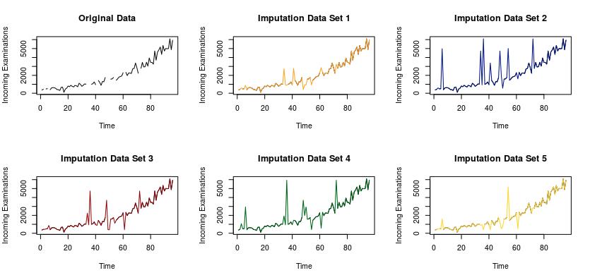
The graph on the top left of the visualization depicts the original data set with the missing values. Each of the following 5 data sets include the imputed values for the missing values. There are advanced statistical methods that can be used to determine which of these models is significantly better than the others. One such method could be to withhold a portion of your original data, a testing set, and impute those values. Ideally we could iterate through this process hundreds, if not thousands of times. Once you have imputed the values from your test sets, you can fit a linear model to your imputed vs. actual examination counts for each of the 5 imputation sets. Then determine which model has the highest R2 to determine which is the best. For the purposes of this pilot study it was decided to use these visualizations to determine that the imputation data set 1 is the best. The imputed values from data set 1 were then added to the Abbeville data to complete the data set, which was then used for the construction and training of the forecasting models.

Data-Analytic Approach

After the data were cleaned and missing values appropriately accounted for, we began the construction of our two forecasting models. We wanted to create two models so that we would be able to compare the output, and determine which would be most effective in predicting cardiovascular examinations. The data for the Abbeville HC is in the form of a time series, which means that there are counts of an event occurring over a period of time. The models that we constructed are both tailor-made for handling time series, which will help us to ensure that our predictions are as accurate as they can be.

First, we wanted to analyze the time series to ensure that conditions were met and to determine which models we should use. The following graph shows the amount of incoming cardiovascular examinations in Abbeville.

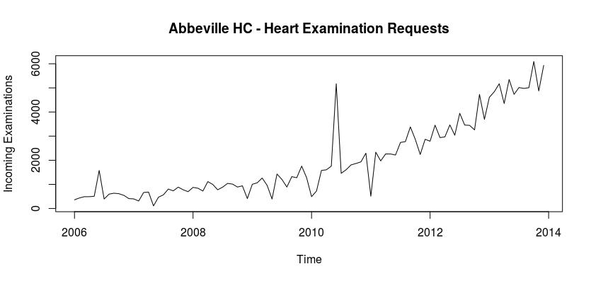
As we can see the number of examinations from January of 2006 to December of 2013 shows a positive trend, and the number of examinations began to increase more drastically around 2011. We then decomposed the time series in order to determine if there is a season or trend component associated with the series. The following visualization contains the decomposition.

# Seasonal Decompisition
labbevilleTS <- log(abbevilleTS)
plot(labbevilleTS, ylab = "log(abbevilleTS)")
fit <- stl(labbevilleTS, s.window= "period") #decomposes time-series
plot(fit, main = 'Decomposed Abbeville Time Series')
fit$time.series #components for each observation

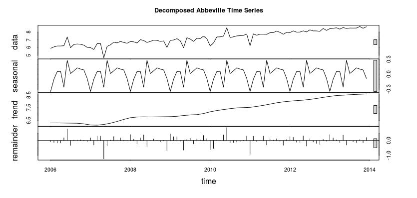
As you can tell from the visualization there is a seasonal and trend component associated with this time series. Therefore we are able to use our forecasting models, as they require the data be seasonal.

Forecasting Models

Model 1 – Holt-Winters Exponential Smoothing

The first model was created using Holt-Winters Exponential Smoothing. Within Holt-Winter smoothing we have three smoothing parameters; alpha, beta and gamma. Alpha controls exponential decay for the level, beta controls exponential dcay for the slope and gamma controls exponential decay for the seasonal component. Using the forecast library in R, we can calculate the best parameters for our model. The parameters that we obtained are: alpha = 0.1648, beta = 1e-04 and gamma = 0.0012.

library(forecast)
fit1 <- ets(log(abbevilleTS), model = "AAA")
fit1
accuracy(fit1)
pred <- forecast(fit1,12)
pred
pred.csv <- as.data.frame(pred)
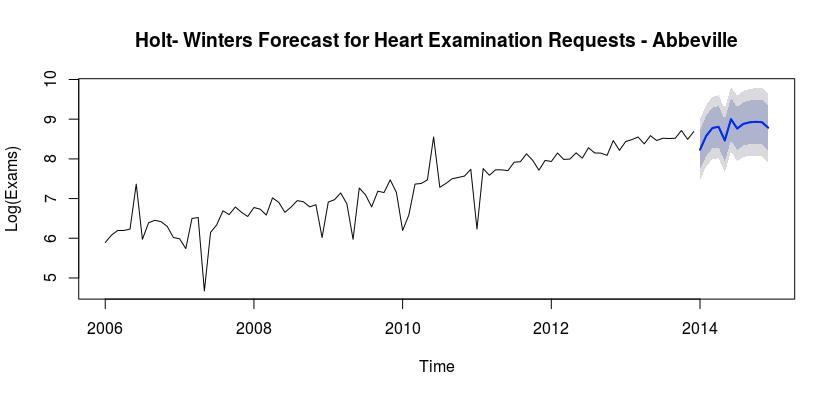
plot(pred, main="Holt- Winters Forecast for Heart Examination Requests - Abbeville",
     ylab = "Log(Exams)", xlab= "Time")
pred$mean <- exp(pred$mean)
pred$lower <- exp(pred$lower)
pred$upper <- exp(pred$upper)
p <- cbind(pred$mean, pred$lower, pred$upper)
dimnames(p)[[2]] <- c("mean", "lo 80", "lo 95", 'hi 80', 'hi 95')
p

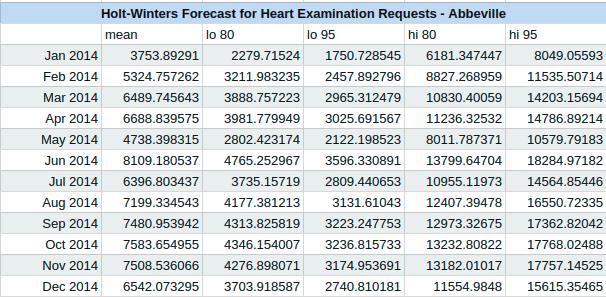
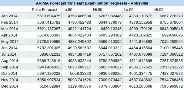
Using the forecast package in R we also obtain an AIC measure for the accuracy of our model. For this model the AIC = 273.4772. We are interested in predicting the next twelve months using our model, and when we do we obtain the results in the following chart. The chart has a mean estimate for the number of examinations in each month, followed by both an 80% and a 95% confidence interval for the number of examinations in each month.

The following graph depicts the cardiovascular exams for the Abbeville hospital, with our predicted counts for the year of 2014, using Holt-Winters exponential smoothing.

Model 2 – Autoregressive Integrated Moving Average (ARIMA)

The second model that we chose to use was an Autoregressive Integrated Moving Average, or ARIMA. We first checked the stationarity of the time series, and found that it is sufficient. We were able to again utilize the forecast package in R and use the auto.arima function to fit an ARIMA model to our data. Using the function we determined that we should use an ARIMA(0,1,1) model to forecast the next twelve months. We also recorded an AIC value of 1486.18. The following is the output of our forecast.

# Transforming Time series and assessing stationarity
library(forecast)
library(tseries)
plot(abbevilleTS)
ndiffs(abbevilleTS)
dabbeville <- diff(abbevilleTS)
plot(abbevilleTS)
adf.test(abbevilleTS)

# Fitting an ARIMA model
fit2 <- auto.arima(abbevilleTS)
fit2
arima.forecast <- forecast(fit2, 12)
accuracy(fit2)
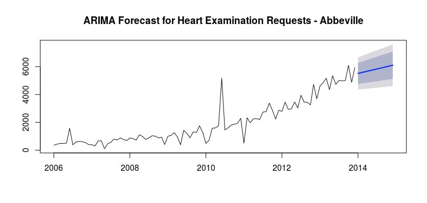
plot(forecast(fit2,12), main="ARIMA Forecast for Heart Examination Requests - Abbeville")

The following graph depicts the cardiovascular examination requests for the Abbeville HC, with our predicted results for the year 2014 from our ARIMA model.

Results

Based on the two models that we were able to create, the Holt-Winters Exponential Smoothing model has a much lower AIC. We can also use the Mean Absolute Error (MAE) to determine the accuracy of both of these models. The MAE for model 1 is 0.262 and the MAE for model 2 is 354.0396. Therefore the first model is more accurate for this situation. As such, we can see that there will be more cardiovascular examinations in 2014 than in 2013. There will also be a spike in June, as well as a lower period in May.

Conclusions and Recommendations

After examining the predictions made with our Holt-Winters model, we can see how this data analytic approach to the staffing of Fargo’s Health Centers will increase revenue for the company by reducing costs and fines for late examinations. We can do this by ensuring that there are enough doctors staffed in the Health Centers to be able to handle the amount of examination requests that will occur. In cases where we need to be more conservative in our staffing, we can take the lower bound of our 80% confidence interval to ensure that we have at least enough doctors to cover that. We will need to be aware of the ethical implications that can arrive from introducing such an optimized schedule model. We will need to be able to live with some lesser optimized scheduling models, to allow our doctors to know their schedule in advance and be able to take time-off. We will be able to apply this model to each Health Center individually, which will enable more accurate predictions.

In order for us to implement this approach there are a few suggestions that we have. The first has to do with the quality of the data. If the data that is used to train the model for each individual Health Center contains many missing value, then the accuracy of the imputation will suffer. For each individual Health Center, we would suggest that extensive work be done to eliminate errors in the data to minimize the ratio of missing values to non-missing values. In addition to overall data quality, the accuracy of the model would be improved greatly if we were able to improve the granularity of the data. The second recommendation that we have is to implement a more statistical approach to selecting which imputation data sets we should use to train our models. This is something that we will be able to do once we begin building the models for each individual Health Center. The third suggestion that we have is to use this predictive model as a foundation for a scheduling tool. This tool would idealistically utilize the forecasting model to predict when there will be a fluctuation of examination requests. If we improve the granularity of the data then the tool would be able to automatically alert a Health Center when they anticipate a need for more doctors.