Mountain Pine Beetle Analysis

Introduction and Problem Background

This project was completed for the B.S. - Statistics program through Brigham Young University

The mountain pine beetle (MPB), is an insect that is found most prevalently in mature pine trees - specifically in the western United States. These beetles typically play an important role in the ecology of an ecosystem, by focusing their attacks on weakened trees they assist in the development of a younger, more healthy forest. Due to the onset of dry conditions and warmer summers, these beetles have been affecting tree mortality rates in conifer forests - such as ponderosas and lodgepole pines. These MBP outbreaks have cause much damage in different regions of the western United States. Researchers are interested in determining what factors contribute most to an area being subject to one of these outbreaks. If we are able to determine the relationships between certain factors and if the area is infested with mountain pine beetles, we will be able to then use statistical modeling to predict in which areas future infestation may occur.

In order to more fully understand this relationship, researchers have obtained data from an annual aerial detection survey conducted by the Colorado State Forest Service (CSFS). The gridded area in the left panel of Figure 1 displays the region of interest for this study.

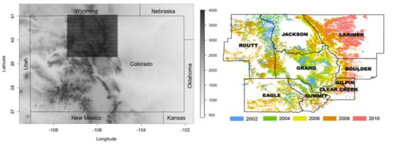
The data set that we have obtained from the CSFS contains the information collected in these annual surveys. The variables that are explained are the following: Is the region infested with pine beetles(Infested - “No”=0 and “Yes”=1), the average January minimum temperature in degrees C(January), the average August maximum temperature(Augustmax), the angle of mountain slope(Slope), the elevation in feet(Elev), the mean annual precipitation in inches(Precip), and an indicator of what region the area is in(region).

In order for us to determine what type of model is viable to use, and to determine if our data are appropriate to use such a model, we need to explore the data and establish some underlying assumptions. Due to the fact that we have a binary response variable (whether or not an area is infested) we will not be able to use a traditional multiple linear regression model. The model that we would need to use is a logistic regression model, which is based on a variable with a Bernoulli distribution. If we attempted to use a different type of model to predict on this data set, we would obtain a number that is not 0 or 1 - which is uninterpretable. When we use a logistic regression model we are able to predict the probability that an area is infested. We have constructed the following visual representations, to assist us in our base-understanding of the data-set. These graphic visualizations help us to know if it is appropriate to use a multiple linear regression model to analyze our data.

  for (i in 1:5){
    scatter.smooth(mpb[,i], mpb$infested, ylab="Infested", xlab=colnames(mpb[i]), col="dark grey", ylim=c(0,1))
  }

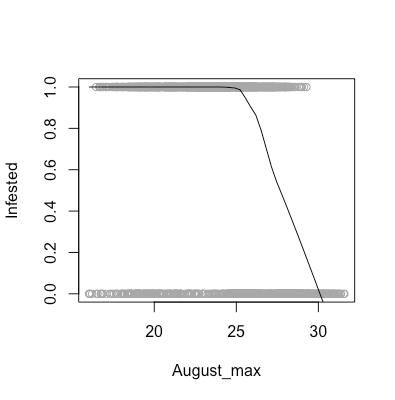
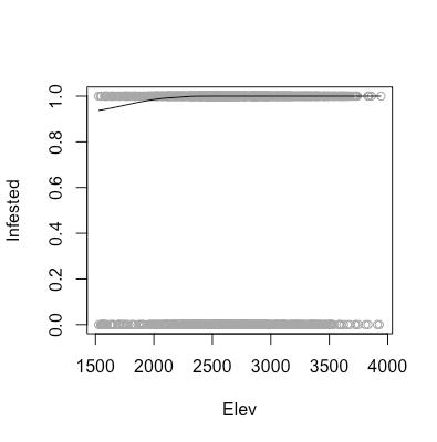
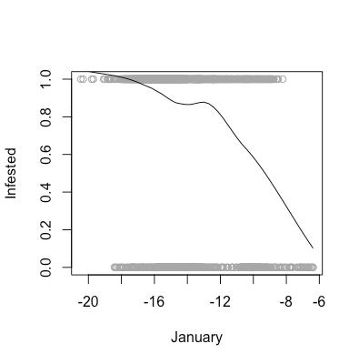
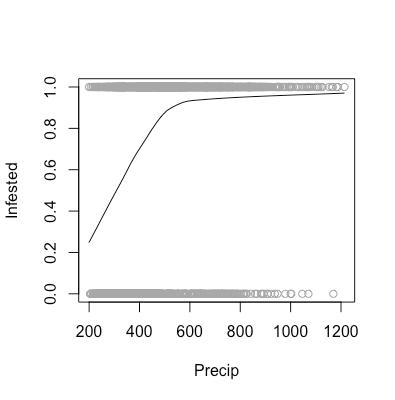
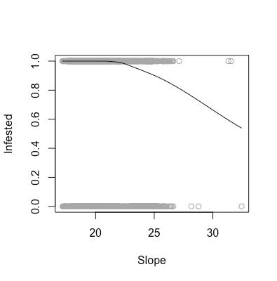
As aforementioned, there are certain assumptions that need to be met in order for us to feel comfortable using a logistic regression model to analyze our data. These assumptions are that our data need to linear in log-odds (monotone in probability), as well as the observations need to be independent. As shown in the above scatter plots, we can see that our data are indeed monotone in probability, and we are willing to assume that one area being infested does not affect the infestation status of another area.

Statistical Modeling

Because the necessary conditions for logistic regression are met, we can now determine which variables need to be included in the model and consequently construct the model based off of those variables. There are multiple methods and techniques that can be used in variable selection, two of the main selection techniques are the Akaike Information Criterion(AIC) and the Bayesian Information Criterion(BIC). When trying different combinations of variables, we can also choose various methods in order to determine the best variables to include. These methods are exhaustive-selection, forward-selection, and backward-selection. The exhaustive approach tests every possible combination of variables to find the best model. Forward selection starts with no variables in the model, adds the best 1, and then the 2nd best variable and so on – until it has constructed the best model. Backward selection is just the opposite, where it starts with all possible variables and removes the worst until the most optimized model is constructed.

Due to the fact that our current data-set that we are working with only contains data with 14 variables, we can use an exhaustive approach and test every single combination of variables (Note: As the size of the dimensions of a data-set increase, the plausibility of using an exhaustive approach decreases. This is when either a forward or backward step selection method should be utilized). We then obtained the best model using AIC and the best using BIC, both with the exhaustive approach. The differences between the two models were extremely small, and so we used our intuition to select the BIC model. The reason for this selection is that BIC is known for simplifying a model, and keeping the most important variables in the model. Therefore, we know that the variables that we are selecting have a significant effect on the probability of an area being infested with beetles.

vs.res.aic <- bestglm(mpb,IC="AIC",method="exhaustive", family=binomial) # AIC is more focused on prediction
best.lm.aic <- vs.res.aic$BestModel
sum.aic <- summary(best.lm.aic)
sum.aic
plot(vs.res.aic$Subsets$AIC,type="b",pch=19,xlab="# of Vars", ylab="AIC")
# pseudo r.squared = 1 - residual deviance/null deviance
pseudo.r.squared.aic <- 1 - (sum.aic$deviance/sum.aic$null.deviance)
pseudo.r.squared.aic

vs.res.bic <- bestglm(mpb,IC="BIC",method="exhaustive", family=binomial) # BIC is more based on inference
best.lm.bic <- vs.res.bic$BestModel
sum.bic <- summary(best.lm.bic)
sum.bic
plot(vs.res.bic$Subsets$BIC,type="b",pch=19,xlab="# of Vars", ylab="BIC")
# pseudo r.squared = 1 - residual deviance/null deviance
pseudo.r.squared.bic <- 1 - (sum.bic$deviance/sum.bic$null.deviance)
pseudo.r.squared.bic

best.lm <- best.lm.bic
sum.best.lm <- summary(best.lm)
pseudo.r.squared.best.lm <- 1 - (sum.best.lm$deviance/sum.best.lm$null.deviance)
pseudo.r.squared.best.lm

summary(best.lm)
sum <- summary(best.lm)

The model we constructed is as follows:

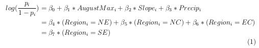
In order to gain a deeper understanding into what this model tells us, we will interpret two of our explanatory variables in context. First, we will interpret the effect of precipitation on the log odds ratio, if we increase precipitation by 1 unit, holding all else constant, then the log odds ratio will increase by \(\beta_3\). Second, we will interpret one of our categorical variables. Due to the fact that we split the “Region” variable into separate indicator variables(NE: “Yes” or “No” etc.), we do not have a region as a part of our baseline level. The baseline for our categorical indicator variables included in the model, is that they are not in that region. For example, we can say that someone in the North East region is \(e^{\beta_4}\) times more likely to be infested by mountain pine beetles.

Results

Now that we know that our model assumptions are met, we can determine to what extent each of our explanatory variables effects the probability of an area being infested with mountain pine beetles.

confint(best.lm)
100 * (exp(confint(best.lm))-1)

The following table contains 95% confidence intervals for the values of each of our coefficients within our fitted model.

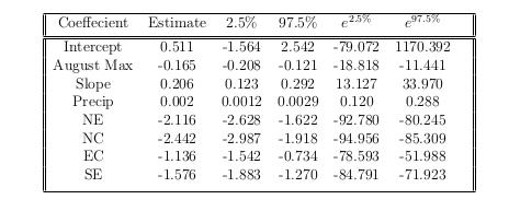
Using the same logic that was used in the previous section, we can interpret these values fairly easily. We can say for example: We are 95% confident, that as we increase precipitation by 1 unit - holding all else constant - that the chance of a region being infested increasing by an amount between 0.12 and 0.288.

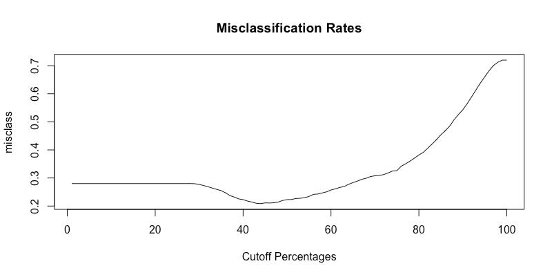
Now that the model has been fitted, we can determine how well it does at predicting the probability of an area being infested with beetles. The method that we can utilize to determine how well the model predicts, is to use cross-validation to determine a misclassification rate. Essentially, we will take out a handful of data points, and use the rest of our data to predict those points. Misclassification occurs when we predict a region to be infested when it actually was not - or predict that it is not infested when it actually was. After performing these cross-validations, we were able to determine a proper threshold value. A threshold is essentially the probability value we will use as a cutoff in determining whether to classify a region as being infested or not. The following graph displays the misclassification rates for the different possible cutoff values. The threshold value we obtained was 0.434343 - or 43.43%.

thresh <- seq(0,1,length=100)
misclass <- rep(NA,length=length(thresh))

for(i in 1:length(thresh)) {
  #If probability greater than threshold then 1 else 0
  my.classification <- ifelse(pred.probs>thresh[i],1,0)
  # calculate the pct where my classification not eq truth
  misclass[i] <- mean(my.classification!=mpb$infested)
}
#Find threshold which minimizes miclassification
threshold <- thresh[which.min(misclass)]

plot(misclass, type="l", xlab="Cutoff Percentages", main="Misclassification Rates")

As we look at the graphic, it is clear that this value is the value that minimizes the number of misclassification.

We have constructed the following table to help us gain insight into how well our model classifies regions as being infested or not.

predfor <- ifelse(pred.probs > threshold, 1, 0)
table(predfor, mpb$infested)
addmargins(table(predfor, mpb$infested))

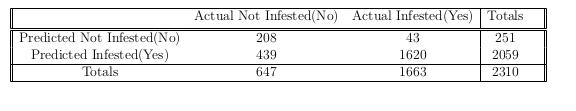
The table is formally known as a confusion matrix, and enables us to calculate four different metrics to help us gain this understanding. The four measurements are: sensitivity - the percent of true positives, specificity – the percent of true negatives, positive predictive value – the percent of correctly predicted yes’s, and negative predictive value – the percent of correctly predicted no’s. These values are easily calculated from the confusion matrix, and are: 97.41%, 32.15%, 78.68%, and 82.87% respectively. These values show that our data do well of classifying our predictions, so we feel confident using our model to classify regions. We also calculated a pseudo-$R^2$, which helps us understand how well our model fits our data. The value we obtained was 0.1583486, which means that 15.8% of the variability in log-odds probability of being infested is explained by our model. This is not the best pseudo-\(R^2\), but it is sufficient.

Predictions

With a logistic regression model that has all assumptions met, the model can be used to predict for all regions, or for one region specifically. The methods used in these predictions are fairly simple, and essentially we can take the characteristics of an area of interest and plug them into the model to obtain a probability that the region will be infested by beetles.

We received a prior request to predict the probability of pine beetle infestation in a particular area. The area that we are interested in predicting for is located in the South East region, has a slope of 18.07, and an elevation of 1901.95.

##  Area characteristics: south east region, slope=18.07, aspect= 175.64, elevation = 1901.95
year <- c(2017, 2018, 2019, 2020, 2021, 2022, 2023, 2024, 2025, 2026)
January <- c(-13.98,-17.80,-17.27, -12.52,-15.99,-11.97,-15.75,-16.19,-17.87,-12.44)
August_max <- c(15.89,18.07,16.74,18.06, 18.23, 15.81, 16.85, 16.51, 17.84, 16.96)
Precip <- c(771.13, 788.54 ,677.63, 522.77, 732.32, 615.96, 805.90 ,714.57 ,740.50 ,801.22)

next.ten <- data.frame(year, January, August_max, Precip)
next.ten

predict.frame <- data.frame(SE="Yes", NE = "No", NC = "No", NW = "No", EC="No", WC="No", SC="No", SW="No",
                      Slope=18.07, Elev=1901.95, January= next.ten$January,
                      August_max= next.ten$August_max,Precip= next.ten$Precip)
pred.log.odds<- predict.glm(best.lm,newdata= predict.frame)
pred.prob <- as.data.frame(exp(pred.log.odds)/(1+exp(pred.log.odds)))
log.odds <- predict.glm(best.lm,newdata=predict.frame,se.fit=TRUE)
int.low <- log.odds$fit - qnorm(0.975)*log.odds$se.fit
int.up <- log.odds$fit + qnorm(0.975)*log.odds$se.fit
pred.int <- exp(cbind(int.low,int.up))/(1+exp(cbind(int.low,int.up)))
pred.int

names(pred.prob) <- c("pred.prob")
out <- data.frame(next.ten$year,pred.int, pred.prob)
names(out) <- c("Year", "Lower Bound", "Upper Bound", "Predicted Prob")
out

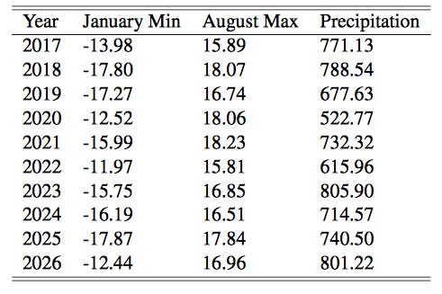
The following table contains forecasts of the maximum August temperatures, minimum January temperatures, and precipitation for the next 10 years.

After performing our calculations, we were able to obtain the following probability predictions for each year, as well as a 95% confidence interval for each year’s predictions. We have collected them in following table:

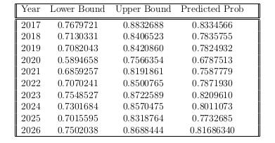
As is clearly visible in the table above, every single one of the 95% confidence intervals is substantially greater than our threshold value of .4343. This means that we are 95% confident that this area will be infested by mountain pine beetles as soon as the year 2017. We would highly recommend the CSFS to concentrate their efforts on this location so as to possibly prevent this infestation, because we are 95% confident this area will be infested.

Conclusions

After conducting our analysis, we have made a few conclusions. First, we have determined which factors, from the ones we were given, have an effect -positive or negative- on determining the probability of an area being infested by mountain pine beetles. These factors are: maximum temperature in August, precipitation, slope, and whether the region is in the NE, NC, EC, or SE regions or not. Through our findings we established these relationships, and can go forward with the knowledge that these relationships are an actuality. Second, we established that our model successfully classifies whether or not a region will be infested with mountain pine beetles. We do have a certain amount of uncertainty, but the fact that 97.5% of the areas truly infested with beetles were predicted as such is a great indicator of the predictive capabilities of our model. We are confident in the abilities of our model to predict which areas will be infested.

Going forward there are a few steps that can be taken, so as to improve the abilities of our logistic regression model. Our first suggestion is to improve the measurements that are being taken into account for forecasting weather conditions. We believe that it is possible that we can improve these measurements, by possibly collecting more detailed temperature data, it is possible wind speed measurements could help determine if the wind is causing beetles to take the easier route, and thus influencing where they are infesting. Another aspect of the research that could be improved is how the data were collected. For the data set received for this analysis, the data were collected via aerial surveys. If we were able to collect data from the ground, then that will increase the reliability of the data. There are numerous possible variables that could be included, and before further studies it would be appropriate to consult with experts in the field. Another possible improvement could be to split the areas up into even smaller regions, allowing us to pinpoint more exactly what factors cause a region to be more likely to be infested.