Predicting Loan Defaults with Logistic Regression

Section 1: Executive Summary

This analysis was conducted with the purpose of optimizing the profit from loans for the bank by predicting the outcome of a potential loan. We are interested in predicting the likelihood that a potential customer will have a ‘good’ or a ‘bad’ outcome on their loan, which in turn will result in whether or not the loan is paid back to the bank.

During the course of the analysis we determined which type of model should be used, which variables we should include into that model, as well as we validated the model to determine the accuracy of the predictions. The detailed methods can be found throughout the remainder of the report. The model that was used to predict the outcome of these loans is called a logistic regression model. This type of model can take many different predictor variables into consideration, and ultimately the outcome is the likelihood of a certain event occurring, in this case whether the outcome of a loan is ‘good’ or ‘bad’. We went through the variables that were given in the original data set and were able to determine which would be the best predictors of loan outcomes. Once we had the model constructed we were able to determine the accuracy of the model through a method known as cross-validation. In this method we create a testing data set and a training data set as subsets from the original data. The training data is used to determine the coefficients of the model and then we use that model to ‘predict’ the outcomes of the testing set. We then compare the accuracy of our model, whether we correctly predicted the outcome of the loan as ‘good’ or ‘bad’. Using the model we accurately predicted the outcome of the loan almost 80% of the time.

Ultimately the goal of this analysis is to be able to create a model which optimizes the amount of profit that the bank receives. With a logistic regression model the output is a proportion between 0 and 1, and the classification value is the point at which we consider the outcome to be a ‘good’ loan or a ‘bad’ loan. The default value in this type of analysis is 0.5, but quite often the optimal classification value for accuracy is different than 0.5. We were able to determine that the optimal classification value for accuracy is 0.58. We also conducted this experiment with profit, to determine which value would lead to the most profit. In this case the optimal classification value for profit was the same as the optimal classification value for accuracy. This means that if the output prediction for any potential customer is above 0.58 we would predict that they would ultimately have a ‘good’ loan outcome and vice versa for those who’s output value is below 0.58. When this value is utilized, in conjunction with our previously stated model, we are able to optimize the profit from the 50,000 loans to $2,787,819.

We suggest that the bank adopts this model in determining which potential customers should be approved for loans. It should be noted that due to the fact that there are unforeseen factors which could effect the outcome of a loan, the bank should utilize this model in conjunction with traditional underwriting techniques. If this takes place, we can cut down on the number of unprofitable loans for the bank and drive profit forward.

Section 2: Introduction

For the purpose of this analysis, we are interested in predicting the likelihood that a potential customer will have a ‘good’ or a ‘bad’ outcome on a loan. We have a dataset containing data on 50,000 loans that will assist in the creation of our prediction model. In order to use this data for our model it will need to be cleaned and prepared for the analysis. In order to predict the likelihood of defaulting on a loan, we will use a logistic regression model. The reason that this model is the most appropriate, is because the outcome we are trying to predict is a binary response, either they will default or they will not. Throughout this report we will document the steps of the data cleansing, analysis, model preparation and implementation.

Section 3: Preparing and Cleaning the Data

In order for us to proceed with our analysis, the data that we have will need to be prepared and cleaned. The first step in doing this is to create one single response variable, which will be used in our logistic regression model. This variable needs to be binary, and will represent whether a loan was a ‘good’ loan or a ‘bad’ loan. In order to create this variable we needed to transform the original variable ‘status’. First we removed loans that had not been resolved, because they will not be able to give us any information on whether a loan was considered ‘good’ or ‘bad’. Next we combined the remaining status values into those two categories. This was done with the understanding that if a loan had been ‘charged off’ or had ‘default’ as the status it was considered a bad loan.

We then needed to address the issue of missing values within the data set. There are many different techniques and approaches that can be taken when it comes to dealing with missing values, such as; Complete Case Analysis, Multiple Imputation, Simple (non-stochastic) Imputation among others. Complete Case Analysis is performed by completely deleting any row with one ore more missing values. Simple Imputation is performed by replacing all missing values with a single decided value (such as the mean, median, mode). In multiple imputation, the missing values are imputed by Gibbs sampling. If the data are missing completely at random, meaning that the chance of the data being missing is unrelated to any of the variables involved in our analysis, a complete case analysis and multiple imputation are both good options. We determined that for the sake of this analysis we would use a complete case analysis because, to the best of our knowledge, the data are missing completely at random. After cleaning and subsetting the data we had 34,655 loans and there were only 384 loans that were missing some form of information - which is only 1.1%. Thus we can use complete case analysis to delete these rows and our model will remained unbiased, and will essentially just be a slightly smaller sample of loans.

###################################
library(lmtest)
library(MASS)
library(GGally)
library(bestglm)
library(DataExplorer)
require(HH)
require(leaps)
###################################

The next step in preparing the data was to eliminate variables that would not be useful as predictors. Due to the fact that we are lacking in the domain understanding of this data, there were only a few variables that we were able to eliminate non-statistically that would not be useful as predictors. These variables were ‘loanID’,’totalPaid’, and ‘employment’. LoanID is obviously not important in prediction. TotalPaid is the amount of money that was paid on a loan, and thus is not able to be determined until after a loan is issued. Employment is the job title for the potential customer, and has 21,401 levels. This variable is too broad and will not be able to prove useful as a predictor. In order to trim down the number of variables to the variables that would be the most efficient in predictions, we built a version 1 model with all of the variables. In this model we conducted the Wald test at an alpha = 0.05 level on whether the coefficients for each of the variables was equal to 0, or in other words whether or not there was a relationship. We decided to keep the variables that have a significant relationship.

# Create Response Variable
loans <- subset(loans,!(loans$status %in% c('Current', 'In Grace Period', 'Late (31-120 days)', 'Late (16-30 days)', '')))
loans$status.new <- factor(ifelse(loans$status %in% c('Charged Off','Default'), 'Bad','Good'))
# Eliminate unneccesary variables(totalpaid collected after and employement title factor w/21401 levels), will use variable selection method later
loans <- subset(loans, select = -c(employment, loanID, status))
# Missing values
#list the rows that have one or more missing values
missing.vals <- loans[!complete.cases(loans),]
nrow(missing.vals)
nrow(missing.vals)/nrow(loans)
## plot_missing(loans)

# Complete Case Analysis
loans.clean <- loans[complete.cases(loans),]


## Variable Selection

r.lm <- lm(status.new~., data = loans.clean)
null <- lm(status.new~1, data = loans.clean)
sf.lm <- step(null, scope = list(lower = null, upper = r.lm), direction = "both")
summary(sf.lm)

## Variables with significant relationship at alpha = .05
updated.loans <- subset(loans.clean, select = c(amount, term, payment, grade, debtIncRat, reason, delinq2yr, inq6mth,
                                                openAcc,revolRatio, totalAcc, totalRevLim, accOpen24, totalRevBal, totalIlLim,
                                                status.new))

Section 4: Exploring and Transforming the Data

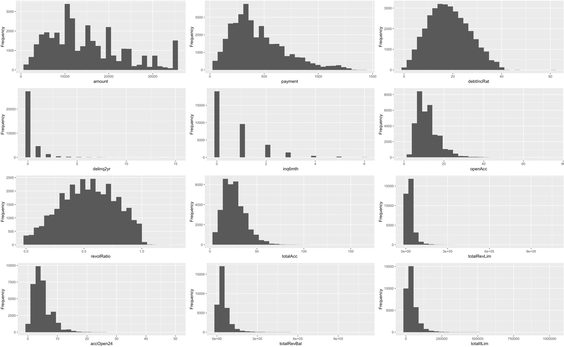
After our data set was cleaned and prepared for analysis, we explored the data to look at the predictor variables, as well as look for trends or needed transformations. The below plot shows the histograms for each of the quantitative variables that we have kept. As you can see there are multiple variables that are very right-skewed.

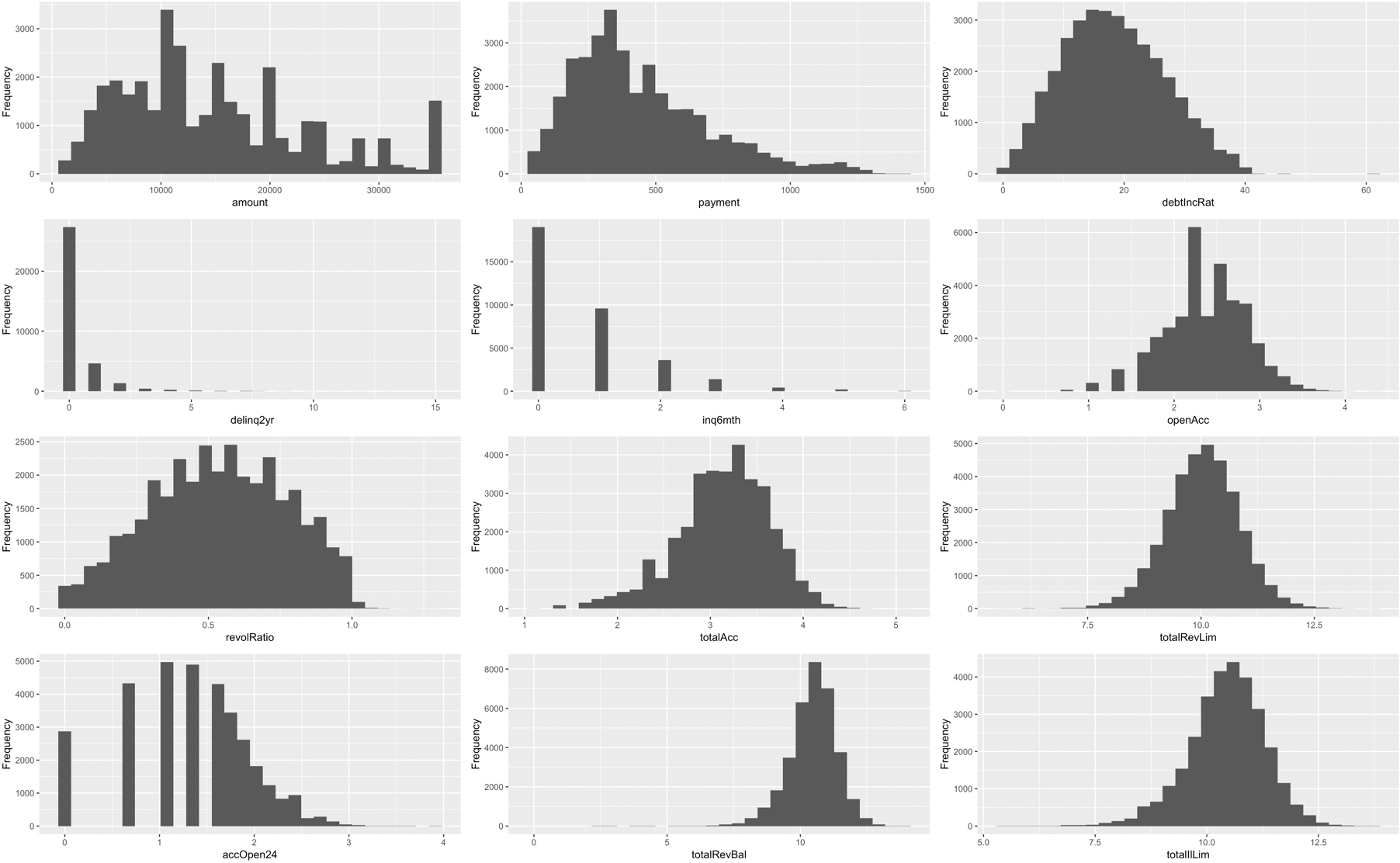
In order to address the skewness of these predictor variables, they were all transformed with a log transformation. The following is the same plot, but including the transformed values. As you can see the variables are no longer as skewed.

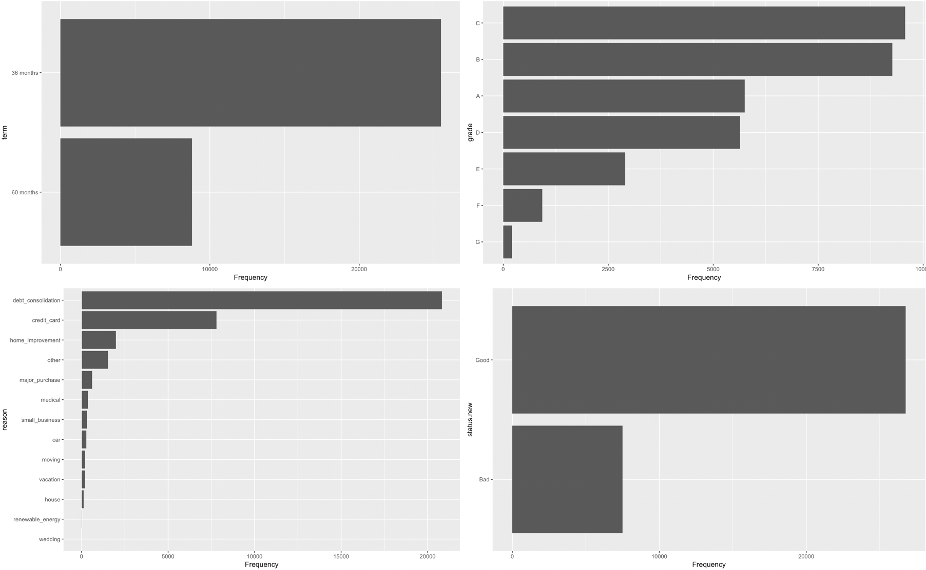
We also created bar charts to explore the categorical variables within the dataset. As you can see in our data there were more good loans than bad loan, more 36 month loans than 60 month loans, the most common reason for loans was for debt consolidation, and the most common grades were C and B.

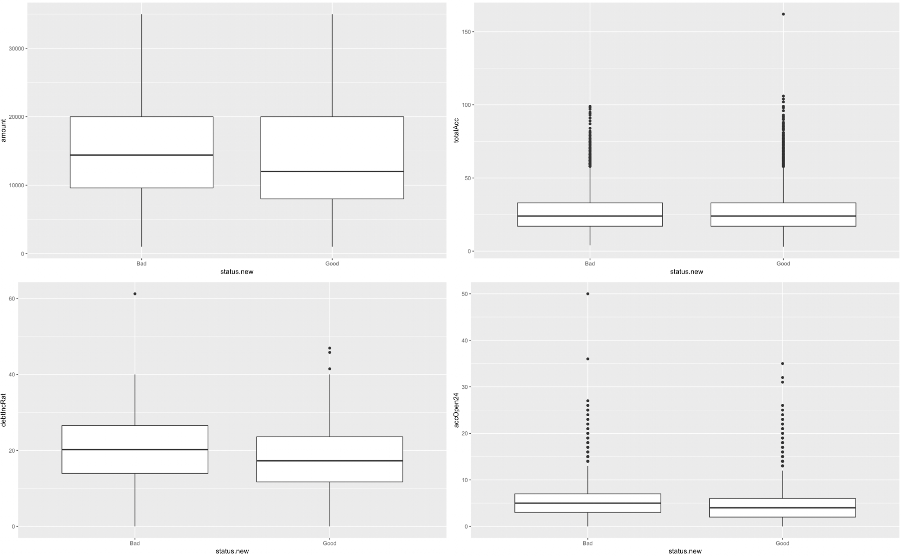
We finally wanted to determine in a visual matter, if there was a relationship between good or bad loan status and some of our variables. The following graphs depict some of these relationships. While there are not huge differences for these 4 predictor variables specifically, there are some differences for good and bad loans. All of the predictor variables were inspected graphically, but these 4 appeared to have the strongest relationships.

library(ggplot2)

multiplot <- function(..., plotlist=NULL, file, cols=1, layout=NULL) {
  library(grid)

  # Make a list from the ... arguments and plotlist
  plots <- c(list(...), plotlist)

  numPlots = length(plots)

  # If layout is NULL, then use 'cols' to determine layout
  if (is.null(layout)) {
    # Make the panel
    # ncol: Number of columns of plots
    # nrow: Number of rows needed, calculated from # of cols
    layout <- matrix(seq(1, cols * ceiling(numPlots/cols)),
                    ncol = cols, nrow = ceiling(numPlots/cols))
  }

 if (numPlots==1) {
    print(plots[[1]])

  } else {
    # Set up the page
    grid.newpage()
    pushViewport(viewport(layout = grid.layout(nrow(layout), ncol(layout))))

    # Make each plot, in the correct location
    for (i in 1:numPlots) {
      # Get the i,j matrix positions of the regions that contain this subplot
      matchidx <- as.data.frame(which(layout == i, arr.ind = TRUE))

      print(plots[[i]], vp = viewport(layout.pos.row = matchidx$row,
                                      layout.pos.col = matchidx$col))
    }
  }
}

g <- ggplot(updated.loans, aes(status.new,amount))
p1 <- g + geom_boxplot()
g2 <- ggplot(updated.loans, aes(status.new, debtIncRat))
p2 <- g2 + geom_boxplot()
g3 <- ggplot(updated.loans, aes(status.new, totalAcc))
p3 <- g3 + geom_boxplot()
g4 <- ggplot(updated.loans, aes(status.new, accOpen24))
p4 <- g4 + geom_boxplot()
multiplot(p1,p2,p3,p4, cols = 2)

Section 5: The Logistic Model

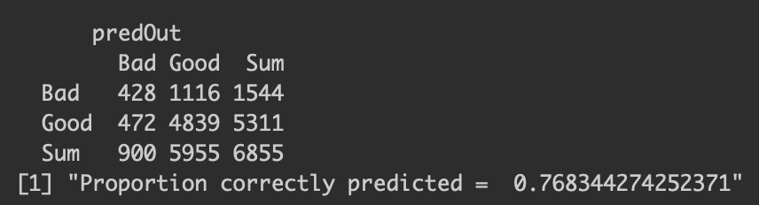
After exploring the data and ensuring that the necessary transformations have been applied, we proceeded to construct the first-order logistic regression model from the variables chosen in the previous section. In order to train the model we randomly select 80% of the loans to be used for the model. We then performed cross-validation on the remaining 20% of the data to determine the accuracy of the model. The table below is a contingency table that compares the predicted values for the 20% test data to the actual outcome of those loans. As the table tells the model correctly predicted 76.83% of the loans in the test set as ‘good’ or ‘bad’ loans.

set.seed(1234)
sample <- sample.int(n = nrow(updated.loans), size = floor(.8*nrow(updated.loans)), replace = F)
train <- updated.loans[sample,]
train <- subset(train, select = -c(totalPaid))
test <- updated.loans[-sample,]


train.mod <- glm(status.new~., data = train, family = 'binomial')

predTest <- predict(train.mod, test)  # get predicted probabilities

threshhold <- 0.5  # Set Y=1 when predicted probability exceeds this
predOut <- cut(predTest, breaks=c(-Inf, threshhold, Inf),
                labels=c("Bad", "Good"))

cTab <- table(test$status.new, predOut)
addmargins(cTab)

p <- sum(diag(cTab)) / sum(cTab)  # compute the proportion of correct classifications
print(paste('Proportion correctly predicted = ', p))

Section 6: Optimizing the Threshold for Accuracy

After constructing the model we wanted to determine the optimal threshold to ensure that our predictions are the most accurate. The default threshold value is set at .5, meaning that if the predicted probability of a long is above .5 then we would classify that loan as ‘good’ and vice versa if it is below .5 we would classify it as ‘bad’. We conducted an experiment with 100 different possible threshold values from 0-1, and determined which value had the lowest misclassification rate. After conducting this analysis is was determined that the optimal threshold for model accuracy is 0.5758. This would say that for the predicted probabilities, anything above 0.5758 would be classified as a ‘good’ loan and anything below would be a ‘bad’ loan.

pred.probs <- predict.glm(v2.mod,type="response")
thresh <- seq(0,1,length=100)
misclass <- rep(NA,length=length(thresh))

for(i in 1:length(thresh)) {
  #If probability greater than threshold then 1 else 0
  my.classification <- ifelse(pred.probs>thresh[i],'Good','Bad')
  # calculate the pct where my classification not eq truth
  misclass[i] <- mean(my.classification!=updated.loans$status.new)
}
#Find threshold which minimizes miclassification
threshold <- thresh[which.min(misclass)]

Section 8: Summary of Results

In summary, the logistic regression model for classifying predictions of loans as ‘good’ vs ‘bad’ will be most accurate and enable the highest profits if a threshold value of 0.5757 is used. While using this value we were able to predict ‘good’ and ‘bad’ loans with roughly 80% accuracy.